How to lock cells in Excel
Lock in on your Excel skills
Sign up for breaking news, reviews, opinion, top tech deals, and more.
You are now subscribed
Your newsletter sign-up was successful
It’s in your best interest to find out how to lock cells in Excel, especially when you’re often handling complicated or extensive Microsoft Excel worksheets at work. After all, handling a spreadsheet with several rows and columns, not to mention hundreds of filled in cells, can get a little confusing. And, mistakes can happen – someone could accidentally drag one cell over the other or one person could delete the contents of a cell without noticing.
Whether it’s those or it’s simply you not wanting the rest of the team to make changes to a particular column or row, knowing how to lock cells in Excel will come in extremely handy sooner or later. Luckily Microsoft designed its whole Office suite very meticulously – so that every single detail is covered, including allowing users to lock individual cells for protection without fuss.
We’re here to show you just how easy it is. Here’s how to lock cells in Excel, whether you’re a Windows 10 user or a macOS supporter.
Article continues below1. How to lock cells in Excel
It doesn’t matter whether you’re a Windows 10 or a macOS user. The steps on how to lock cells in Excel are pretty much the same, even if the interfaces might look slightly different. Just follow our instructions below, and you’ll be locking those cells like a pro in no time.
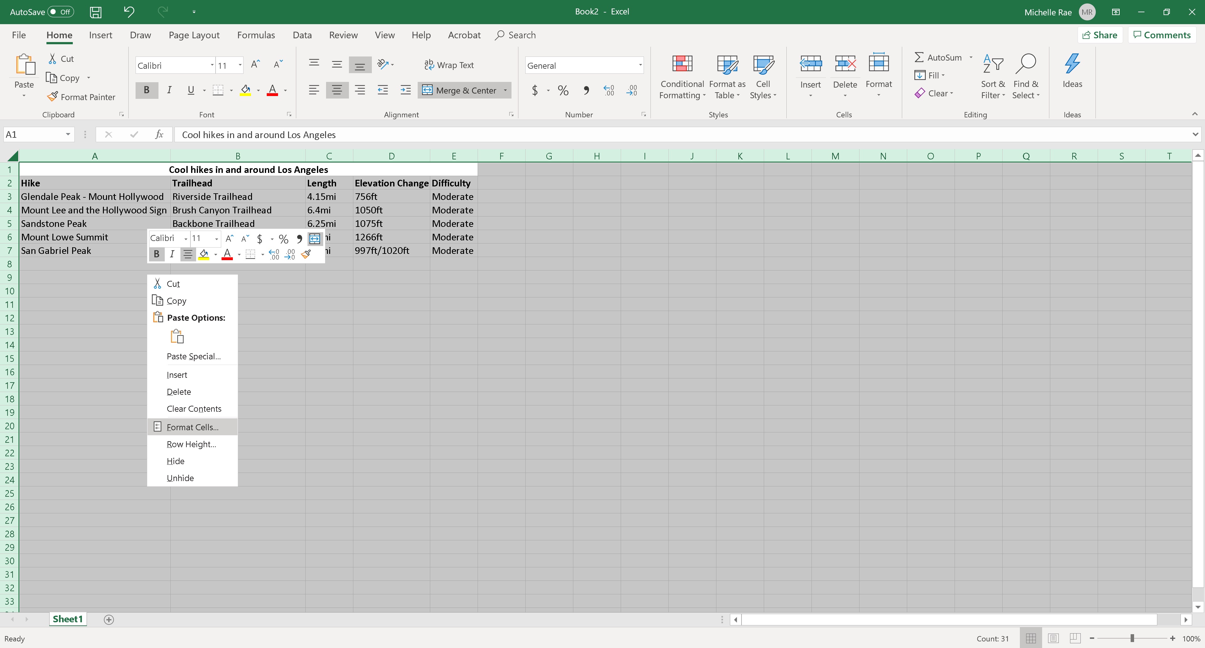
Step 1: Select all cells in the worksheet.
By default, Microsoft Excel has every single cell on a new worksheet set to lock. This doesn’t mean that the cells are not editable at default; only that if you decide to lock the whole worksheet, you can do so quickly and without the added steps.
If you need to lock only a few specific cells in your worksheet, you need to make sure first that then the whole sheet is unlocked.
Sign up for breaking news, reviews, opinion, top tech deals, and more.
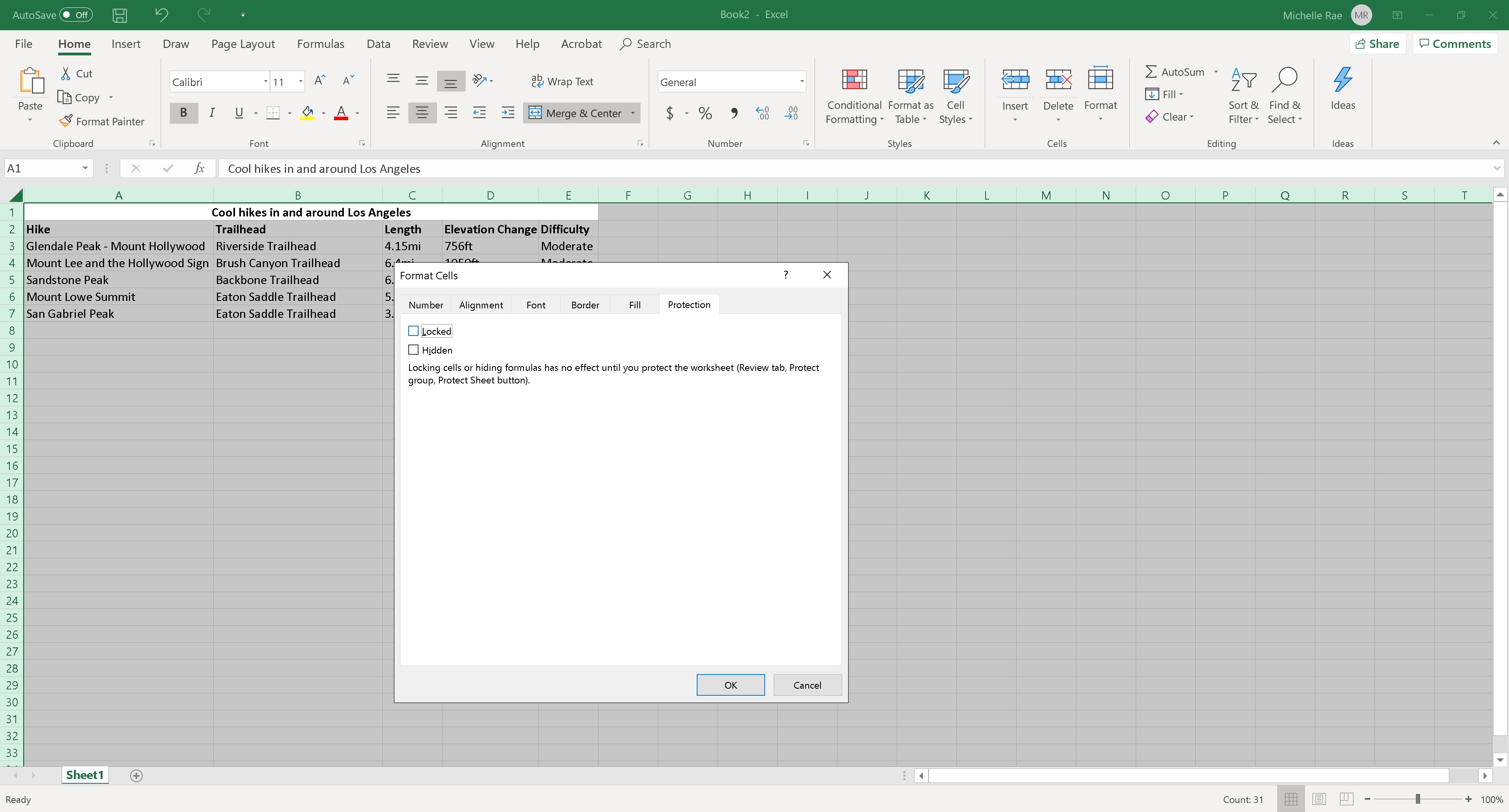
Step 2: To unlock the whole sheet, right-click on Windows 10 (two-finger tap on macOS). Then click on Format > Protection. Deselect or uncheck “Locked” and click OK.
Essentially, this unlocks every cell on that worksheet.
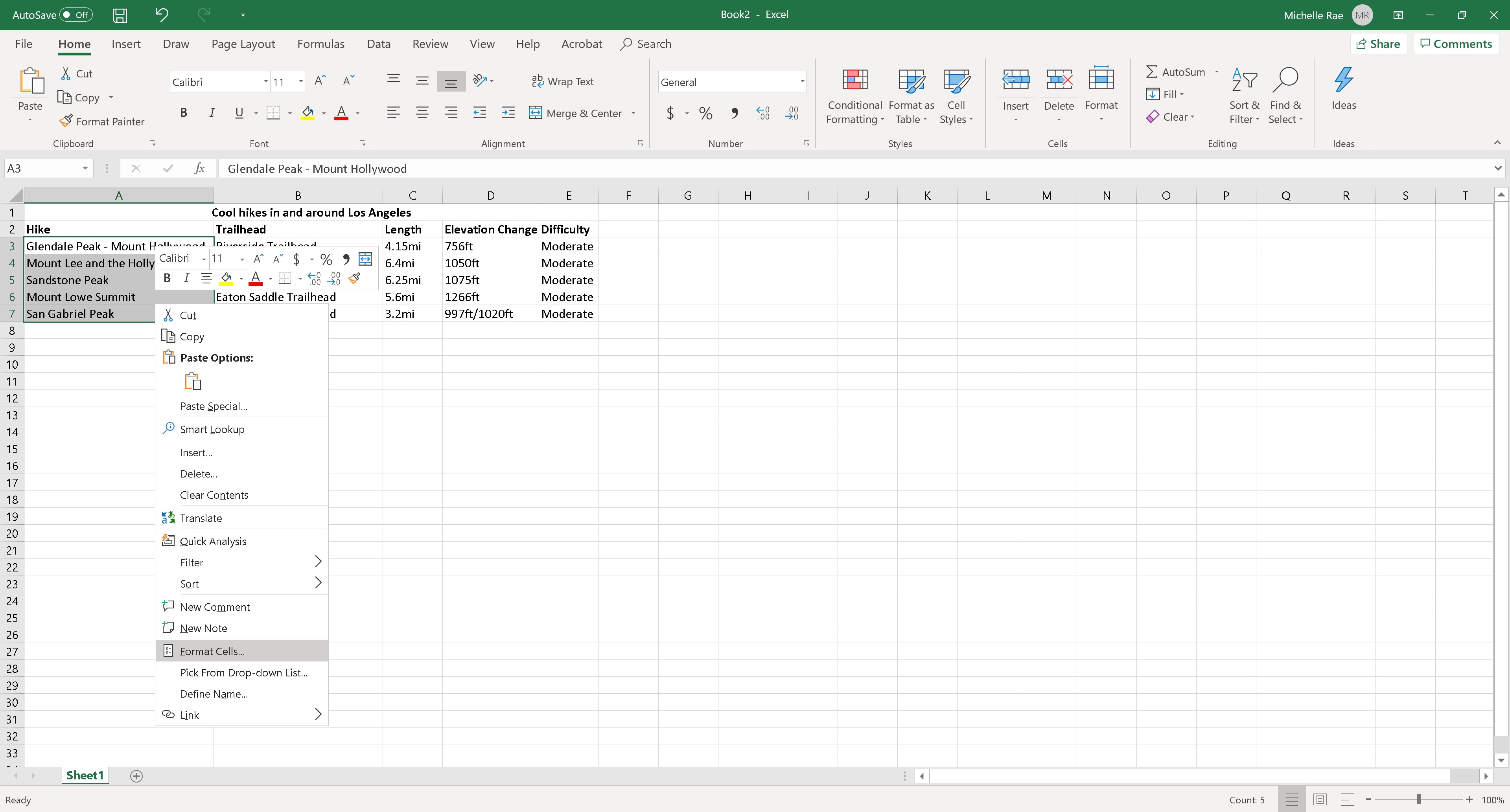
Step 3: Select all the individual cells you want to lock.
You may select entire rows or columns, or specific cells. To select specific cells that are not next to each other, hold down the Command key on macOS or Control key on Windows 10 as you select every cell individually.
Step 4: On one of the selected cells, right-click on Windows 10 (two-finger tap on macOS). Then click on Format > Protection again.
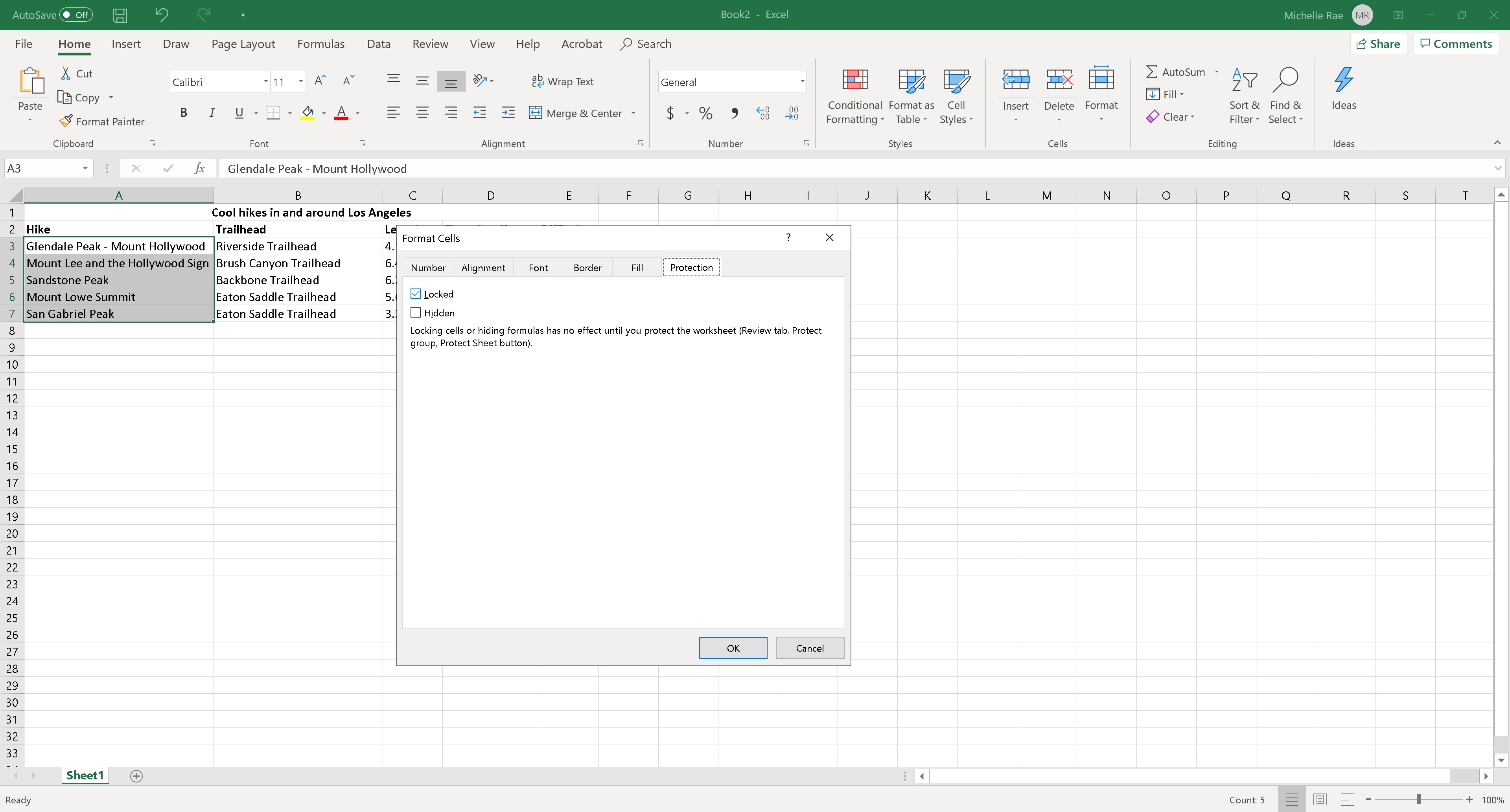
Step 5: This time, tick off “Locked” and click OK.
This tells Excel that you want those specific cells to be locked. This step, however, doesn’t exactly lock the sheets. To lock those sheets, you still have to tell Excel to protect the worksheet.
Step 6: On the main menu, go to the Review tab and click Protect Sheet.
A dialogue box will open to let you select a few options and also set a password. Set a password, if you need to.
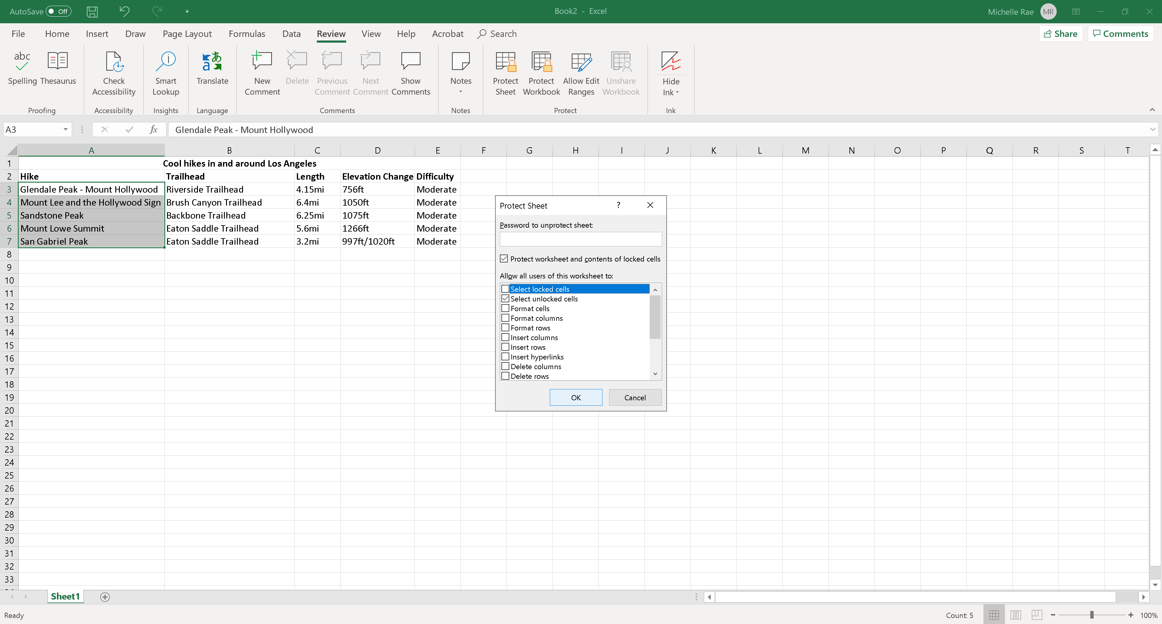
Step 7: Only tick off “Select unlocked cells” and uncheck everything else.
This effectively locks the cells you’ve selected, but also leaves everything else unlocked for editing.
Images credit: Michelle Rae Uy

Michelle Rae Uy is the former Computing Reviews and Buying Guides Editor at TechRadar. She's a Los Angeles-based tech, travel and lifestyle writer covering a wide range of topics, from computing to the latest in green commutes to the best hiking trails. She's an ambivert who enjoys communing with nature and traveling for months at a time just as much as watching movies and playing sim games at home. That also means that she has a lot more avenues to explore in terms of understanding how tech can improve the different aspects of our lives.