Sign up for breaking news, reviews, opinion, top tech deals, and more.
You are now subscribed
Your newsletter sign-up was successful
Join the club
Get full access to premium articles, exclusive features and a growing list of member rewards.
Replicating nature
Sadly, there's no way we can mimic 20 billion neurons with 10,000 connections each, but there are several interesting things we can do with much less firepower.
Way back in 1957, Frank Rosenblatt modelled a single neuron with something he called a 'perceptron', and used it to investigate pattern recognition. Unfortunately, the perceptron was unable to recognise even simple functions like XOR (proved formally by Marvin Minsky and Seymour Papert in 1969) and so it was abandoned in favour of something called multilayer feedforward networks.
Article continues belowNevertheless we can use many of the concepts associated with the perceptron later on.

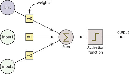
Above shows a standard perceptron. We have a set of inputs on the left-hand side. Each input has a 'weight' associated with it. Each input signal (which is a floating-point value, positive or negative) is multiplied by its weight (another floating-point value).
All of these products are summed. If the sum exceeds a threshold value (generally 0), the perceptron outputs 1 (or 'true'). If the threshold is not exceeded, the perceptron outputs 0 (or 'false').
This test is known as the activation function. To help with the process, another fixed input is usually provided (known as the 'bias'). This models the propensity of the perceptron to fire in spite of the values of its inputs. The bias is normally 1 and will have its own weight.
Sign up for breaking news, reviews, opinion, top tech deals, and more.
All this is very well, but where do the weights come from? The inputs are obviously provided by us in some form, but who provides the weights?
Look at it like this. Suppose we want a perceptron to calculate the same result as the AND operation. There will be two inputs to this perception, A and B. Each input will be constrained to two possible values, 0 and 1. If both A and B equal 1, the perceptron should output 1; otherwise it should output 0.
We have to determine three weights here: the weights for A and B and the bias. Once we have these, we should be able to run the perceptron, and it should produce the correct outputs for the four possible combinations of input. The only way of doing this is to train the perceptron.
First thing we need is a set of inputs and their expected outputs. For our simple example, we have four training sets: 1 and 1 gives 1, 0 and 1 gives 0, 0 and 0 gives 0, and 1 and 0 gives 0.
We set all weights to zero. Note that this perceptron will produce the right answer for the last three training sets automatically. The first set will produce an error (it should produce 1, but gives 0, an error of 1).
What we do now is to modify the weights to take account of the error. We make use of a new constant called the learning rate (a number between 0 and 1) and modify each weight to add a term that's proportional to the error value, the learning rate and its input value.
Start off with a high rate (say, 0.8). We then let the perceptron learn using its training materials until the weights stabilise. If the weights don't converge after a few iterations, the perceptron is possibly oscillating around the solution, so it's best to reduce the learning rate.
If the weights never converge, then the function being modelled by the perceptron cannot be recognised.
After Minsky and Papert showed that a single perceptron couldn't solve some simple patterns, research stagnated. Eventually, efforts shifted to studying a multilayer system instead.
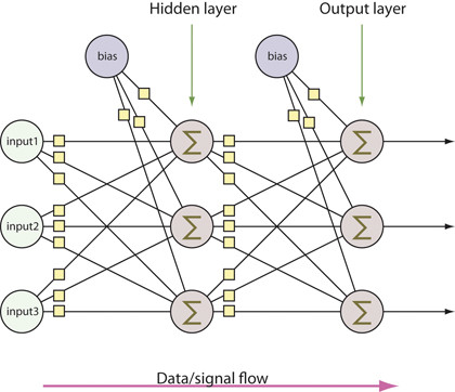
The first such system was called the feedforward neural network. In a multilayer system of perceptrons, there are at least three layers: the input layer, the hidden layer and the output layer. The latter two layers are the perceptrons. Below shows an idealised view of such a network.

Notice that the data or signals travel one way, from the input layer to the output layer, hence the term feedforward. There are no cycles here. The hidden layer is shown here to have three perceptrons, but this is by no means a fixed number.
Indeed, the number of hidden perceptrons is yet another 'knob' to twiddle to tune the neural network (the weights being the only knobs so far). The number of output perceptrons is a function of the pattern you're trying to recognise, so if you were trying to perform OCR on digits, you might have 10 output perceptrons, one for each digit.
Notice that all of the input signals feed into all of the perceptrons in the hidden layer, and all the outputs from the perceptrons in the hidden layer feed into the perceptrons in the output layer. If an input for a perceptron is not needed, the weight will be set to zero.
Finer tuning
The big issue with this neural network is in training it. The most successful algorithm devised is known as the back-propagation training algorithm, but it requires some changes.
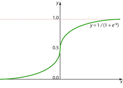
The first change is that the perceptron should output not just a 0 or a 1, but a floating-point value between 0 and 1. This will in turn require the perceptron to use a different activation function, one that's a curve instead of being a step function.
The functions used here are known as sigmoid functions. These are S-shaped functions with asymptotes at 0 and at 1.
Below shows the standard one that's used: f(x) = 1/(1+e-x), but others include the hyperbolic tangent (tanh) or the error function (erf).

If a perceptron calculates a very large sum of its weighted inputs, it'll output a value close to 1; if the sum is very large and negative, it'll output a value close to 0; if it's close to 0, the perceptron will output a value around 0.5.
Once these changes have been made, the network is 'differentiable'; that is, it's possible to calculate gradients. The gradients we want to calculate are to help us change the weights due to a training error: a steep gradient for an input signal means a larger change in its weight, a more gradual gradient means a smaller change.
The gradient also gives a direction (upwards or downwards), so we know whether to add or subtract the correction term. And all this means that, despite the much greater complexity of a feedforward neural network, training it still only requires a few cycles.
Obviously you have to pre-calculate a catalogue of training sets (so, for example, if you were creating a neural network to recognise the digits using OCR, you'd use as many different variants of the digits using all the fonts you could find), and those training sets would be fed into the network as often as needed until the weights converged.
Of course, this time around, you would have the extra knob to twiddle: the number of hidden perceptrons. Here there are no real guidelines apart from the more of them there are, the longer it will take to train the network, and you may not gain any more accuracy.
Generally, though, you would aim for having at least as many hidden perceptrons as you have perceptrons in the output layer.
-------------------------------------------------------------------------------------------------------
First published in PC Plus Issue 288
Liked this? Then check out The past, present and future of AI
Sign up for TechRadar's free Weird Week in Tech newsletter
Get the oddest tech stories of the week, plus the most popular news and reviews delivered straight to your inbox. Sign up at http://www.techradar.com/register
 Become a TechRadar Insider


