How your sat-nav works out the best route
Sign up for breaking news, reviews, opinion, top tech deals, and more.
You are now subscribed
Your newsletter sign-up was successful
Join the club
Get full access to premium articles, exclusive features and a growing list of member rewards.
It's now time for the second algorithm: determining the optimal route from the current position (defined as a point with some latitude and longitude values) to a destination (defi ned in the same way).
An immediate prerequisite is the map. The map in a sat-nav is a peculiar beast. It's first and foremost a vector map – it consists of a set of data that is primarily in vector format. Since it comprises a set of vectors, the display part of the sat-nav unit must draw the vectors (that is, the roads, mostly) on the screen at runtime, and take account of the orientation and position of the car at that moment.
Compare this with the mosaic maps (or tiled maps) used by mapping websites like Google Maps. Here the map is served up as a pre-calculated set of square images (tiles) which are then painted onto the screen by the browser. The tiles sent to the browser are those needed for the current resolution of the map and for the area covered by the browser's window. The tiles are always oriented in the same manner, with north to the top.
Think of the vectors in the vector map in a sat-nav as straight road segments. They consist of two positions (beginning and end) defined by latitude and longitude, and will have further information tagged with them, such as the name of the street or road and whether the road is a major thoroughfare such as a motorway or A road or a smaller one like a backstreet or one-track lane. A road then consists of several segments placed end to end.
Now the fun starts. We have two points of interest: the current location and the destination. We have a map that's defined as a large set of vectors. We have to use the latter to calculate the most optimal route to go from the current location to the destination.
The usual algorithm used is Dijkstra's algorithm for finding the least-cost path between two nodes in a weighted graph or network. To recap, a graph is a data structure that consists of a set of vertexes (sometimes known as nodes) with links (usually known as edges) between them. A weighted graph has a cost associated with each edge.
If you think about it, a vector map is such a graph. The vectors are edges, and the ends of each vector can be thought of as the nodes. Since a road will consist of a set of vectors joined end to end, you can visualise that most nodes in the map just have two edges. Without any real loss of generality, we'll assume that the starting and ending locations are defined by latitude/longitude pairs and happen to be the ends of vectors (that is, we don't want to get into the geometric algorithm that determines inside which vector a particular point can be found).
Sign up for breaking news, reviews, opinion, top tech deals, and more.

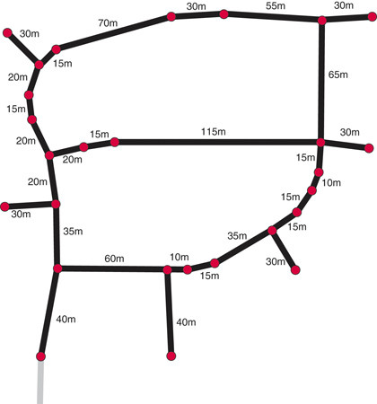
Above shows a simplified example of a vector map of the Pinewoods estate where I live (the lower left node, coloured grey, continues out of the estate). I've marked the lengths of each vector, delimited by the red nodes, to the nearest 5m. The cost of each vector is a function of the way it has been tagged and also of its length. We can imagine that motorways and A roads have a low 'cost' value whereas streets and C roads have a high 'cost'.
The length of a vector also has a cost, one that is proportional to the length of the vector. Dijkstra's algorithm is intended to calculate what's known as the shortest path tree from a given node, or in other words, to reorganise the nodes in the network into a tree such that, if you follow the links from the initial node (the root of the tree) to any other, you will traverse the path with the smallest cost.
We're not particularly interested in the full tree though, since the number of vertexes and edges in any sat-nav city map is going to be huge, and, in planning the route, the sat-nav will be (or rather, should be) ignoring the vast majority. Dijkstra's algorithm also fails in the sense that all nodes are equally 'important', whereas we know that the nodes in the direction we want to travel are going to be more important than others.
What we need is a directed version of Dijkstra's algorithm, one that takes into account the fact that the sat-nav map database is, well, a map. Certain vectors in the map just won't be considered; they're in the opposite direction, for example.
Somehow we need to encode nodes that are closer to the target as being more significant than nodes that are further away.
The A* algorithm
The algorithm used is called the A* algorithm (pronounced 'A star'). It is a graph algorithm that finds the path with the smallest cost from a starting node to the target node. It was devised by Hart, Nilsson and Raphael in 1968.
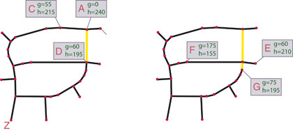
A* uses two values when considering a node to be added to the smallest cost path: the actual smallest cost of reaching the node from the start node – usually called g – and a heuristic estimate of the distance from the node to the target node, usually called h.
The simplest heuristic we can use is a simple 'as the crow flies' distance to the target, taking no account of any roads, corners or whatnot. A further value called f is calculated as g + h. (Let's note in passing that Dijkstra's algorithm is equivalent to the A* algorithm with the heuristic h set to 0 for every node.)

This is how it works. (Follow along with Figure 2 as we find the path from A to Z on my vector map.) We set up the path to be empty. For the source node, g is 0, and h is the direct 'crow' distance to the target node. Add it to a priority queue, which is a data structure that releases nodes with the highest priority first.
Our priority here is going to the inverse of the f value – so lower values of f mean higher priority. Go into a loop until the priority queue is empty or we've found the target node (the more preferable outcome). Each time round the loop, remove from the priority queue the node with the smallest f value. Add it to the current path.
Now search through all the nodes that can be reached from this node (that is, find all the vectors that have the current node as an end point). Ignore all nodes that are in the current path. For each of these reachable nodes, calculate their possible g value (it will be the current node's g value plus the edge cost to the other node).
If the node has been 'seen' before (that is, it's somewhere in the priority queue), this possible g value may be smaller than the previous one, in which case we can replace it. Calculate the h value and therefore the f value, and, if the node is not in the priority queue, add it.
Of course, if the node from the priority queue is the target, we add it to the current path and stop as we've solved the problem. If we run out of nodes in the priority queue, it means that the target node is not reachable from the start node. We've failed to find a path.
Of course, in the real world, we wouldn't expect this to happen (unless we were trying to get from London to the Isle of Man with a sat-nav that doesn't 'know' about ferries). After we have the shortest route (or, rather, the route with the smallest cost), the software in the sat-nav unit then has to display it on the screen, either as a 2D map or, more commonly nowadays, as a 3D projection of the map, and then update it as you travel along.
But that, as they say, is an article for another day.
-------------------------------------------------------------------------------------------------------
First published in PC Plus Issue 292
Liked this? Then check out Street to screen: how sat-nav maps are made
Sign up for TechRadar's free Weird Week in Tech newsletter
Get the oddest tech stories of the week, plus the most popular news and reviews delivered straight to your inbox. Sign up at http://www.techradar.com/register

 Become a TechRadar Insider


