
 Become a TechRadar Insider


Excel is a great tool to use to create a quiz for work or play. It can track correct and wrong answers, and keep a running score of your progress. You can make up your own list of questions or do as we did and find some on the web to use.
Our movie questions came from www.adviceopedia.com. We’ll show you how to create the quiz, how to write the formulas that track progress and how to keep the answers away from prying eyes.
Structure the workbook
To start, open a new workbook and rename ‘Sheet1’ and ‘Sheet2’ to read ‘Quiz’ and ‘Answers’. You do this by double-clicking the tab for each sheet and typing the new name.
In cell B1 of the ‘Quiz’ worksheet, type Number of Questions . In cell B2, type Your Score . Across row 4 starting in Column A type: Question, Answer, Result.
Down column A from cell A5 downwards, type the questions, one per cell. Then switch to the worksheet called ‘Answers’ and starting in cell A5, type the answer to the corresponding question on the ‘Quiz’ sheet. Adjust the width of column A so you can read the questions.
Add the formulas
Formulas do all the work of checking answers and keeping score. In cell C5, type this formula:
=IF(B5””,IF(B5=Answers!A5,”Correct”, “Incorrect”),””)
This checks the answer in cell B5 to see if it matches the contents of cell A5 on the ‘Answers’ worksheet. If the answer is correct it places the word ‘Correct’ in the current cell.
If the answer is incorrect, it reads ‘Incorrect’. Copy this formula down column C so it appears opposite each question.
In cell C1, opposite the heading ‘Number of Questions’, type this formula:
=COUNTA(A:A)-1
This will return the number of questions in your quiz.
In cell C2, opposite the words ‘Your Score’, type the following formula to calculate the score, assuming you have less than 4,995 questions in total:
=COUNTIF(C5:C5000,”=Correct”)
Format the worksheet
An easy way to format the worksheet attractively is to select all the cells in the range, starting at A4 and ending with the cell in column C opposite the last question.
Go to ‘Home > Format as Table’, choose a table format and click ‘OK’. Then click ‘Table Tools > Design Tab > Convert to Range’ to remove the unwanted table features.
Select the cells in column B that will contain your answers, right-click and select ‘Format Cells > Protection tab’, deselect ‘Locked’ and click ‘OK’. This will unlock the cells so that data can be entered in them when the worksheet is protected.
Step-by-step: Protect your answers
Step 1:

Hide the sheet containing the answers by right-clicking it and selecting ‘Hide’ from the menu. While this hides the answer sheet, it’s still possible for someone to unhide it, so more work remains to be done.
Step 2:

To protect the ‘Quiz’ worksheet, go to ‘Review tab > Protect Sheet’. Set the dialogue so the only selected option is ‘Select Unlocked Cells’. Type a password to protect the sheet and enter it again when prompted. Users can now only select cells in column B and they won’t see the formulas that indicate where the answers are.
Step 3:

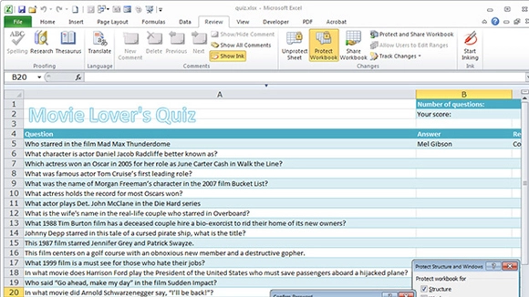
To protect the workbook so the ‘Answers’ sheet itself can’t be unhidden, click ‘Review tab > Protect Workbook’. Select ‘Structure’ and type a password.