Excel tutorial – Sales and commissions

Make your business more efficient with our Excel Tutorial on creating a sales and commission spreadsheet

In this article I am going to show off five top Excel tricks for making your spreadsheets sing and to help edit and refine your sales and commissions spreadsheet.

These tricks make it easier to create spreadsheets that are easy to use and which allow you to get to the heart of the matter immediately. None of them involve any scripting, VBA or macros and once learnt can be applied in any spreadsheet.

The tricks will cover layout and formatting, sorting, highlighting important data and searching for information.

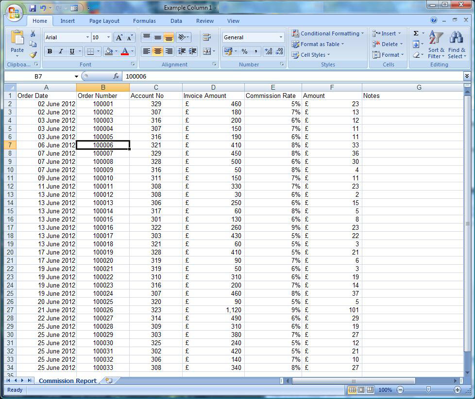
Our working spreadsheet is a very familiar scenario: a list of orders sorted by date with prices and commissions and it looks like the sheet below.

1/ Formatting your spreadsheet

The first thing I want to do is a bit of formatting to make the headers stand out. I get the font, colour and alignment of cell A1 just right.

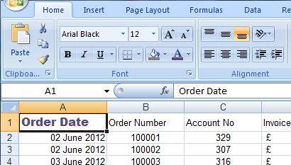
Everyone knows the little format painter icon on the cut and paste panel on the home tab in the ribbon bar. When you click this it picks up the format of the current cell and allows you to paint another cell or range of cells. It only allows you to do this once, if you have lots of different cells you want to format the same way you need to re-click the format painter. With a big spreadsheet this could be a bit 'peck and hunt'. In modern versions of Excel though you can double click the format painter to lock it on. It changes to and stays that way until you next click it. So I can easily format my page.

2/ Editing headlines to fit the page

OK, so each header looks nice but we have another classic spreadsheet problem: the columns are a bit congested, and if I fix that then the data goes off the page.

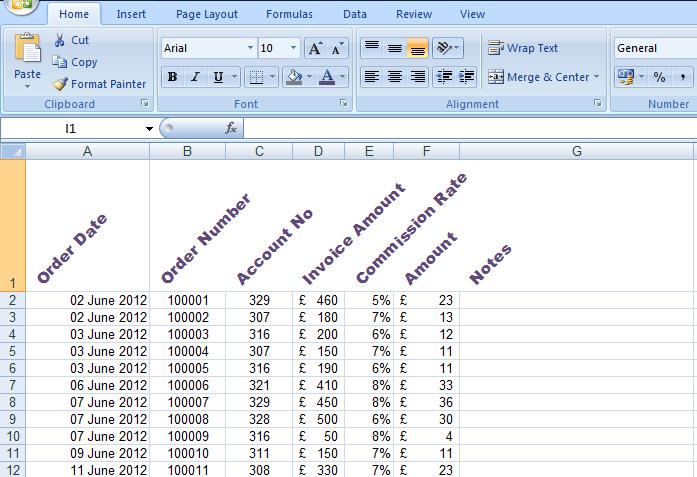
I can solve this problem elegantly using the Orientation button on the Alignment panel on the Home Tab:

It's the little angled 'ab' with an arrow. I select all the headings and use this dropdown to select 'angle counterclockwise'. This tips the column headers on their side and I can now shrink the columns to make the page nice and compact whilst keeping the column headers clear:

3/ Conditional formatting to highlight what's important

The next trick is to highlight the most important bits of information for me eg my commission. To do this we are going to use conditional formatting from the Styles panel on the home tab:

The drop down offers a number of options:

• Highlight Cell Rules
• Top/Bottom Rules
• Data Bars
• Colour Scales
• Icon Sets

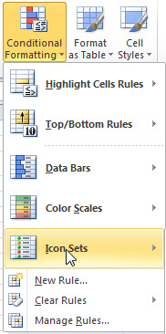
I am going to choose the icon sets option and then the simple traffic lights option. If I select all the commission payments and apply conditional formatting I get:

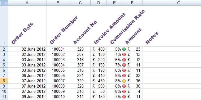
Excel has applied the default rules to the traffic lights:

If I go back and select the menu Conditional Formatting -> Icon Sets -> More Rules we get the rules dialog box:

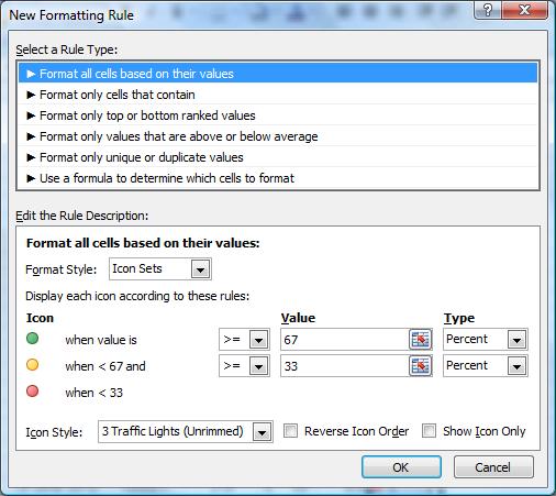
This shows the default rules are green for the top third of values, red for the bottom third and yellow for the middle third.

There is a tricky problem with conditional formatting that trips people up. These conditional rules apply to all the values in the selection at the time the formatting was applied. I need to select all the values and apply the conditional format to them as a group. I want to flag all payments above £40 as green, and all those below £20 as red because they are too small to worry about. The middle set get yellow. We can just select all cells and edit the formula to do that.

4/ Grouping and sorting by a filter

In order to improve my sales performance I need to be able to group all the sales to a single customer account and work out which ones are valuable to me. I am going to do that with the sort and filter function on the sort and filter panel on the data tab.